
💡 Author: Ian Helfrich Edition: First Date: April 2023
Table of Contents
Preface
Acknowledgements
Part I: Foundations of Modern Macroeconomics
Chapter 1 – Introduction to Macroeconomics
Chapter 2 – Macroeconomic Data: Sources, Methods, and Limitations
Chapter 3 – Classical and Keynesian Macroeconomic Models
3.1 The Classical Model: Say’s Law and the Quantity Theory of Money
Introduction to the Classical Model
The Classical Model is an economic framework that emerged during the Enlightenment and has been developed by a number of prominent economists such as Adam Smith, David Ricardo, and John Stuart Mill. The Classical Model is based on the principles of free markets, self-regulation, and limited government intervention. It emphasizes the importance of supply-side factors in determining economic outcomes and assumes that markets will naturally reach equilibrium, ensuring full employment and stable prices.
Historical Context
The foundation of the Classical Model can be traced back to Adam Smith‘s groundbreaking work, “The Wealth of Nations” (1776). Smith, often referred to as the father of modern economics, introduced the concept of the “invisible hand” to describe how the self-interested actions of individuals in a market economy unintentionally benefit society as a whole. He argued that free markets, driven by competition and the division of labor, lead to greater efficiency and prosperity.
David Ricardo, another key figure in classical economics, contributed significantly to the development of the model through his work on comparative advantage, which explained how nations can benefit from international trade by specializing in the production of goods they can produce most efficiently. John Stuart Mill further refined the Classical Model, incorporating ideas such as the law of diminishing returns and the principle of population.
Mathematical Expressions
- Say’s Law: Y = C + I, where Y represents total output, C represents consumption, and I represents investment. According to Say’s Law, total output is equal to the sum of consumption and investment, emphasizing the importance of supply-side factors in determining economic outcomes.
- The Quantity Theory of Money: MV = PY, where M represents the money supply, V represents the velocity of money, P represents the overall price level, and Y represents real output. This equation illustrates the direct relationship between the money supply and the price level, emphasizing the Classical Model’s view on the neutrality of money in the long run.
Detailed Notes, Facts, and Figures for Students to Study
Adam Smith
Adam Smith’s “The Wealth of Nations” (1776) is considered a seminal work in economics and laid the foundation for the Classical Model. Smith’s ideas about free markets, competition, and the division of labor have shaped the field of economics and continue to be influential today.
David Ricardo
David Ricardo’s “Principles of Political Economy and Taxation” (1817) introduced the concept of comparative advantage, which remains a fundamental concept in international trade theory. Comparative advantage explains how countries can benefit from specializing in the production of goods and services they are relatively more efficient at producing.
John Stuart Mill
John Stuart Mill’s “Principles of Political Economy” (1848) incorporated ideas such as the law of diminishing returns and the principle of population, further refining the Classical Model. Mill’s work also emphasized the importance of individual freedom and the role of government in promoting social welfare.
- The Classical Model’s assumptions include:
- rational economic agents,
- flexible prices and wages,
- full employment in the long run, and
- the neutrality of money.
These assumptions underpin the model’s view that markets are self-regulating and efficient.
Critiques of the Classical Model
The Classical Model has been critiqued for its limited applicability to modern economies, particularly in the face of recessions and depressions. The Great Depression of the 1930s, for example, exposed the limitations of the Classical Model and led to the development of Keynesian economics.
Summary of the classical model
The Classical Model is an important economic framework that emphasizes the importance of supply-side factors and the self-regulating nature of markets. While it has been subject to critiques and modifications over time, the Classical Model remains a foundational aspect of economic theory. Understanding its principles, historical context, and mathematical expressions can help students gain a deeper appreciation of the evolution of economic thought and the role of markets in shaping economic outcomes.
Say’s Law: supply creates its own demand
Say’s Law, formulated by the French economist Jean-Baptiste Say, is a central tenet of the Classical Model. It posits that supply creates its own demand, meaning that the production of goods and services generates enough income for consumers to purchase those goods and services. In other words, the act of producing goods and services generates enough purchasing power to clear the market. This idea suggests that economic downturns or recessions are temporary and will eventually self-correct, as producers adjust their output in response to changes in demand.
The Quantity Theory of Money: MV = PY
Introduction to the Quantity Theory of Money
The Quantity Theory of Money is a core concept in the Classical Model, which posits that the total money supply (M) multiplied by the velocity of money (V) is equal to the overall price level (P) multiplied by the real output of goods and services (Y). This theory implies that changes in the money supply have a direct and proportional impact on the price level but no long-term impact on real output or employment. In other words, an increase in the money supply will lead to inflation, but it will not change the overall level of economic activity.

The Classical Dichotomy and the Neutrality of Money
Introduction
The Classical Dichotomy and the neutrality of money are key concepts in classical economics that help us understand the relationship between nominal and real variables in an economy. These ideas are central to the Classical Model, which assumes that changes in nominal variables do not have a lasting impact on real variables in the long run.
- If a central bank decides to double the money supply, the neutrality of money suggests that, in the long run, this action will only lead to a proportional increase in the price level (doubling of prices) but will not affect the real output, employment, or real wages in the economy.
Long-run price flexibility and full employment
The Classical Model assumes that prices and wages are fully flexible in the long run, meaning that they will adjust to changes in supply and demand to ensure market equilibrium. As a result, the Classical Model predicts that the economy will always return to full employment in the long run, as wages and prices adjust to clear the labor market. This view contrasts with the Keynesian Model, which argues that wages and prices can be “sticky” or slow to adjust, leading to persistent unemployment and underutilized resources.
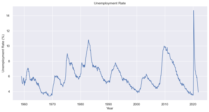
The following graphs show the inflation rate, unemployment rate, and real GDP growth rate over time. The first graph demonstrates the relationship between inflation and unemployment, while the second graph shows the real GDP growth rate. The data covers the period from 2000 to 2021, which includes the Great Recession and the subsequent recovery. Observe how unemployment increased during the recession, and later declined as the economy recovered. Additionally, you can see how the inflation rate fluctuates over time, but it is not directly correlated with the unemployment rate. The real GDP growth rate also shows the contraction during the recession and the subsequent recovery.
These graphs provide a visual representation of the concepts of long-run price flexibility and full employment, as well as the interplay between inflation, unemployment, and real GDP growth in the U.S. economy.
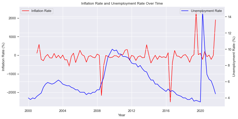


This graph shows an enhanced version of the Phillips Curve, illustrating the relationship between inflation and unemployment rates. Note that the relationship is not as clear-cut as it was in the original Phillips Curve, which is in line with the Classical Model’s assertion that real variables are determined independently of nominal variables.
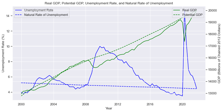
This graph illustrates the relationship between the natural rate of unemployment, actual unemployment rate, potential GDP, and real GDP. The dashed lines represent the natural rate of unemployment and potential GDP, while the solid lines represent the actual unemployment rate and real GDP. The graph demonstrates the concept of full employment and long-run price flexibility, as it shows that in the long run, the economy tends to return to its potential GDP and natural rate of unemployment.
These graphs, along with the explanations provided, offer a more comprehensive understanding of the Classical Model and its key concepts, such as full employment and long-run price flexibility. They also showcase the power of Python and various libraries, such as pandas, matplotlib, and seaborn, to create visually appealing and informative graphics using real-world data from FRED.
Policy implications of the Classical Model
The policy implications of the Classical Model are generally laissez-faire, emphasizing the limited role of government in the economy. According to the Classical Model, government intervention should be minimal, as markets are self-regulating and naturally tend toward full employment and stable prices. Classical economists generally argue that government intervention, such as fiscal or monetary policy, can only have short-term effects on the economy and may even be counterproductive in the long run. They advocate for policies that promote free markets, such as deregulation, low taxes, and minimal government spending.
The Classical Macroeconomic Model, rooted in the works of Adam Smith, David Ricardo, and John Stuart Mill, among others, has had a profound impact on the field of economics and the development of economic policies. This chapter examines the policy implications of the Classical Model, focusing on its main tenets: Say’s Law, the neutrality of money, flexible prices, and full employment in the long run. We will also explore the implications of these principles for fiscal and monetary policies and the role of government intervention in the economy.
Say’s Law and Aggregate Demand
Say’s Law, named after the French economist Jean-Baptiste Say, posits that supply creates its own demand. In other words, an increase in production will result in a corresponding increase in aggregate demand. This principle implies that there is no persistent problem of insufficient demand or overproduction in a market economy, as any increase in output will be matched by an equal increase in demand.
Policy Implications of Say’s Law and Aggregate Demand
Say’s Law suggests that government intervention aimed at increasing aggregate demand is unnecessary, as the economy is self-regulating and will naturally balance itself. This principle has implications for both fiscal and monetary policies, as it argues against the need for government spending, tax cuts, or changes in the money supply to stimulate demand and promote economic growth.
The Neutrality of Money
The Classical Model posits that changes in the money supply only affect nominal variables such as prices and wages, while real variables, like output and employment, remain unchanged in the long run. This concept, known as the neutrality of money, implies that monetary policy has no long-term impact on real economic activity.
Policy Implication: The neutrality of money implies that changes in the money supply will only result in inflation or deflation, without affecting real output or employment. Consequently, central banks and monetary authorities should focus on maintaining price stability rather than attempting to influence real economic activity through changes in the money supply.
Flexible Prices and Full Employment
The Classical Model assumes that prices and wages are fully flexible, adjusting to changes in supply and demand to achieve market equilibrium. This flexibility allows the economy to return to full employment in the long run, as wages and prices adjust to clear the labor market.
Policy Implication: The assumption of flexible prices and full employment in the long run suggests that government intervention to address unemployment is not necessary. Instead, the economy will naturally adjust to reach full employment without any external stimulus. This principle has implications for policies such as minimum wage laws, unemployment benefits, and labor market regulations, as it argues that these interventions may hinder the economy’s ability to achieve full employment.
Fiscal and Monetary Policies in the Classical Model
Given the principles of Say’s Law, the neutrality of money, and flexible prices, the Classical Model has significant implications for the role of fiscal and monetary policies in managing the economy.
Fiscal Policy
The Classical Model suggests that government intervention through fiscal policy is unnecessary, as the economy will naturally achieve full employment and maintain a balanced aggregate demand. Therefore, policymakers should focus on maintaining a balanced budget and avoiding deficit spending, which could lead to inflation and distort the allocation of resources in the economy.
Monetary Policy
According to the Classical Model, changes in the money supply have no long-term impact on real economic variables, making monetary policy ineffective in influencing output and employment. Consequently, the primary goal of monetary policy should be to maintain price stability and avoid excessive inflation or deflation.
Labor Market Policy
The Classical Model posits that flexible wages and prices will allow the economy to return to full employment in the long run. Consequently, classical economists tend to argue against policies that interfere with labor market flexibility, such as minimum wage laws and strict employment protection legislation. However, modern policymakers must weigh the benefits of labor market flexibility against the potential social costs of income inequality, job insecurity, and labor market dualism. Policies that promote worker protection, skill development, and social safety nets can help to mitigate these negative consequences while preserving the efficiency gains associated with flexible labor markets.
International Trade
The Classical Model, particularly through David Ricardo’s theory of comparative advantage, emphasizes the benefits of free trade and specialization for global welfare. This principle has informed the design of modern trade agreements and the liberalization of trade barriers, fostering economic integration and growth. However, the potential distributional consequences of trade, as well as the challenges posed by global imbalances and trade-related externalities, require a comprehensive approach to trade policy that considers both the efficiency gains of free trade and the need for complementary policies to address its potential drawbacks.
Conclusion
The Classical Macroeconomic Model offers essential insights for modern economic policy, emphasizing the importance of market mechanisms, price stability, and the benefits of international trade. However, contemporary policymakers must also recognize the limitations of the Classical Model and consider the role of government intervention in addressing market failures, mitigating the social costs of economic policies, and promoting a stable and inclusive economy. By understanding the modern policy implications of the Classical Model, policymakers can draw on its enduring wisdom while adapting their strategies to the complex and evolving challenges of the global economy.
3.2 The Keynesian Model: Aggregate Demand and the Multiplier
Introduction to the Keynesian Model
The Keynesian Model, developed by the British economist John Maynard Keynes in response to the Great Depression of the 1930s, offers a different perspective on macroeconomic equilibrium than the Classical Model. The main difference lies in the focus on aggregate demand as the primary driver of economic activity and the belief that market forces may not always bring the economy back to full employment in the short run.
Keynes argued that, during recessions, inadequate aggregate demand could lead to involuntary unemployment and that government intervention might be necessary to stimulate demand and restore full employment. The Keynesian Model has been influential in shaping modern macroeconomic policies, including the use of fiscal policy to manage economic fluctuations.
Aggregate demand (AD) from a Keynesian perspective is the total demand for goods and services in an economy at a given price level. It is the sum of consumption (C), investment (I), government spending (G), and net exports (NX), that is, exports (X) minus imports (M). According to the Keynesian Model, changes in AD can lead to fluctuations in output and employment. An increase in AD can lead to higher output and employment, while a decrease in AD can lead to lower output and unemployment.
Involuntary unemployment is a situation where individuals who are willing and able to work are unable to find employment at the prevailing wage rates. This can occur due to a lack of available jobs, a mismatch between the skills of workers and the jobs available, or other structural factors in the labor market. The concept of involuntary unemployment is central to the Keynesian Model, which argues that government intervention may be necessary to stimulate demand and reduce unemployment during economic downturns.
The concept of Aggregate Demand (AD)
Aggregate Demand (AD) represents the total demand for goods and services in an economy at a given price level. It is the sum of consumption , investment , government spending , and net exports , that is, exports minus imports :
According to the Keynesian Model, changes in AD can lead to fluctuations in output and employment. An increase in AD can lead to higher output and employment, while a decrease in AD can lead to lower output and unemployment.
Aggregate demand is the total quantity of goods and services demanded in an economy at a given overall price level at a given time. It is depicted by the aggregate demand curve, which describes the relationship between price levels and the quantity of output that firms are willing to provide. It is often represented as the sum of four major categories:
- Consumption : This is the total spending by consumers on goods and services during a specific period. It is the largest component of AD and tends to increase as income increases.
- Investment : This is the total spending by businesses on capital goods, which are used to produce other goods. It includes spending on new buildings, machinery, and changes in inventory levels. Investment spending is influenced by interest rates and expectations about future economic conditions.
- Government Spending : This is the total spending by all levels of government on goods and services, including public services, infrastructure, and social services. It does not include transfer payments, such as social security or unemployment benefits.
- Net Exports : This is the total spending on a nation’s goods and services by foreigners (exports) minus total domestic spending on foreign goods (imports).
Mathematically, the aggregate demand is represented as:
Mathematical Structure
To understand how aggregate demand functions, it’s helpful to look at its components more closely.
Consumption is typically modeled as a function of disposable income (income after taxes). A simple linear consumption function could be written as:
where:
- is autonomous consumption, or the amount of consumption when disposable income is zero.
- is the marginal propensity to consume, or the change in consumption due to a change in disposable income.
- is national income.
- is total taxes.
Investment can be influenced by many factors, but in the simplest models, it’s often treated as exogenous, or determined outside the model.
Government Spending is also usually considered as exogenous in simple models, determined by the policy decisions of government.
Net Exports can be affected by the relative prices of goods in different countries and the exchange rate. In the simplest models, net exports might be treated as exogenous.
Combining these components gives us a simple model for aggregate demand:
Examples
Let’s suppose we have the following data for an economy:
- Autonomous consumption, billion
- Marginal propensity to consume,
- National income, billion
- Total taxes, billion
- Investment, billion
- Government Spending, billion
- Net Exports, billion (i.e., a trade deficit)
We can plug these values into our aggregate demand equation to find:
billion
The Keynesian Cross and the expenditure multiplier
The Keynesian Cross is a graphical representation of the relationship between aggregate demand (AD) and aggregate output in the short run. It is based on the assumption that the economy is characterized by a consumption function, which depends on disposable income:
Where is autonomous consumption, c is the marginal propensity to consume , is aggregate output, and is taxes.
The equilibrium condition in the Keynesian Model is when aggregate demand (AD) equals aggregate output :
The Keynesian Cross illustrates the expenditure multiplier effect, which arises from the fact that an increase in autonomous spending (e.g., government spending or investment) can lead to a more than proportionate increase in aggregate output. The expenditure multiplier is given by:
Where is the marginal tax rate.
The paradox of thrift and the importance of demand management
The paradox of thrift is a concept introduced by Keynes to illustrate the importance of demand management in an economy. It states that, although saving may be individually rational, an increase in the aggregate saving rate can lead to a decrease in aggregate demand, output, and employment, ultimately hurting the economy as a whole.
This paradox highlights the need for active demand management policies, such as fiscal and monetary policies, to stabilize the economy during periods of insufficient aggregate demand.
The role of fiscal policy in the Keynesian Model
Fiscal policy, which involves the use of government spending and taxation to influence the economy, plays a crucial role in the Keynesian Model. According to Keynesian theory, fiscal policy can be used to stabilize the economy during periods of economic fluctuations by influencing aggregate demand.
- Expansionary fiscal policy: During a recession, the government can use expansionary fiscal policy, such as increasing government spending or reducing taxes, to boost aggregate demand and stimulate economic growth. This policy can help close a recessionary gap and restore the economy to full employment.
- Contractionary fiscal policy: During an economic boom, the government can use contractionary fiscal policy, such as decreasing government spending or raising taxes, to reduce aggregate
- The role of fiscal policy in the Keynesian Model demand and prevent the economy from overheating. This policy can help close an inflationary gap and maintain stable prices.
Fiscal policy in the Keynesian Model is often associated with the use of discretionary policies, which involve active decisions by policymakers to adjust government spending or taxation in response to changing economic conditions. However, it’s important to note that there are also automatic stabilizers, such as progressive taxation and unemployment benefits, which can help stabilize the economy without explicit intervention by policymakers.
In summary, the Keynesian Model emphasizes the importance of aggregate demand in determining economic activity and the need for demand management policies, such as fiscal policy, to stabilize the economy during periods of insufficient or excessive demand. The Keynesian Cross and the expenditure multiplier demonstrate the potential impact of changes in autonomous spending on aggregate output, while the paradox of thrift highlights the potential negative consequences of excessive saving on the economy as a whole.
3.3 The Consumption Function and Investment
- The consumption function: marginal propensity to consume (MPC) and average propensity to consume (APC)
- Determinants of consumption and the life-cycle hypothesis
- The importance of investment in economic growth
- Determinants of investment: interest rates, business expectations, and government policy
- Investment and the accelerator effect
3.4 The IS-LM Model
3.4.1. Introduction to the IS-LM framework
1. Introduction
- Brief History and Importance of the IS-LM Model The IS-LM model is a macroeconomic model that was first introduced by Sir John Hicks in 1937, as an interpretation of John Maynard Keynes’s General Theory. The IS-LM model has been a fundamental tool in macroeconomic teaching and policy making. It provides a simplified framework to analyze the relationship between interest rates, real output in the goods and services market, and the money market.
- Overview of the IS-LM Framework The IS-LM model is a model of aggregate demand that represents the interaction of the “real” economy (Investment-Saving, or IS) and the monetary sector (Liquidity preference-Money supply, or LM). The IS curve represents equilibrium in the goods market, and the LM curve represents equilibrium in the money market. Their interaction determines the equilibrium level of income and interest rate in the economy.
2. IS-LM Model Components
- Goods Market (IS Curve) The IS curve illustrates the equilibrium in the goods market, showing the relationship between the interest rate and the level of income that arises from equilibrium in the goods market. In this market, total spending equals total income (or output).
- Money Market (LM Curve) The LM curve represents equilibrium in the money market, depicting the relationship between the interest rate and level of income that arises from the equilibrium in the money market. In this market, the quantity of money demanded equals the quantity of money supplied.
- Interaction of IS and LM Curves The point where the IS and LM curves intersect represents the short-run equilibrium of both the goods and money markets. At this point, the interest rate and the level of income in the economy are in equilibrium.
The IS-LM (Investment Saving – Liquidity Preference Money Supply) model is a key macroeconomic tool for understanding the interaction between the real and monetary sectors of the economy. Initially developed by John Hicks in 1937 as an interpretation of Keynes’s General Theory, the model has since played a fundamental role in macroeconomic teaching and policy making.
In this lecture, we will examine the IS-LM framework, diving deeper into the theory and mathematics behind it, exploring its historical context and significance, and discussing practical applications.
2.2 IS-LM Model Components
2.2.1 Goods Market (IS Curve)
The IS curve describes the goods market equilibrium where total spending (consumption, investment, and government spending) equals total income or output.
Mathematically, the goods market equilibrium condition (total spending equals total income) is given by:
where Y is income (or output), C is consumption, T is taxes, I is investment, r is the real interest rate, and G is government spending.
In this equation, C(Y – T) represents consumption as a function of disposable income (Y – T), and I(r) is investment as a function of the interest rate. The IS curve is derived from this equation, showing all combinations of Y and r that satisfy the goods market equilibrium.
2.2.2 Money Market (LM Curve)
The LM curve represents the money market equilibrium, where the quantity of money demanded equals the quantity supplied.
The money market equilibrium condition is typically expressed in terms of the liquidity preference theory as:
where M is the nominal money supply, P is the price level, L is the demand for real money balances, Y is income, and r is the real interest rate. L is an increasing function of Y and a decreasing function of r. The LM curve, hence, represents all combinations of Y and r that satisfy the money market equilibrium.
2.2.3 Interaction of IS and LM Curves
The IS-LM model’s equilibrium is defined by the intersection of the IS and LM curves, where both the goods and money markets are in equilibrium simultaneously.
This joint equilibrium can be represented by a system of two equations derived from the IS and LM curves:
The solution to this system of equations gives the equilibrium values of Y (income/output) and r (real interest rate). This intersection represents the short-run equilibrium of the economy.
As we delve deeper into the IS-LM model, we’ll explore shifts in these curves, how they affect equilibrium income and interest rates, and the implications for fiscal and monetary policy. This model provides a powerful framework for analyzing a wide range of macroeconomic phenomena, despite its simplifying assumptions, and will serve as a cornerstone of our understanding of macroeconomics.
3. Assumptions in the IS-LM Model
We’ll now delve into the core assumptions of the IS-LM model and provide mathematical context, practical examples, and aids to facilitate comprehension.
3.1 Closed Economy
The IS-LM model is based on a closed economy assumption, meaning it doesn’t include international trade (exports and imports) or international capital flows. In mathematical terms, we omit the net exports (X – M) component from the national income identity in the goods market:
Here,
- is the total income (output)
- represents consumption
- denotes investment
- stands for government spending
By excluding , we ignore the effects of changes in net exports on income, interest rates, and investment.
Example: In a real-world situation, an interest rate increase might cause capital to flow into the country, appreciating the currency and reducing net exports . With the closed economy assumption, we disregard these effects.
3.2 Short Run Analysis
The IS-LM model focuses on short-run fluctuations, while ignoring long-run factors like technological progress or population growth. It assumes that the price level (P) is fixed or doesn’t change significantly in the short run. This assumption simplifies the model but limits its application to long-run scenarios.
The LM curve, which represents money market equilibrium, is described mathematically as:
Here,
- is the nominal money supply
- is the price level
- is the real money demand, which is a function of the interest rate (i) and income
In this equation, we consider M/P (the real money supply) as fixed in the short run, underscoring the model’s short-run focus.
3.3 Role of Expectations
The basic IS-LM model does not consider expectations about future economic conditions, including anticipated inflation or future income. This can impact current consumption, investment, and money demand.
For instance, consider the consumption function:
Here,
- is autonomous consumption (consumption when income is zero)
- is the marginal propensity to consume
- is disposable income
In this equation, future expectations can affect autonomous consumption . If households anticipate a future increase in income, they might consume more in the present, leading to a rise in .
While the IS-LM model’s simplicity is a strength, these assumptions can limit its applicability. Recognizing these limitations allows us to use the IS-LM model where appropriate and seek more complex models when necessary.
4. Limitations of the IS-LM Model
The IS-LM model has been a fundamental tool in macroeconomic teaching and policy-making. Yet, as with any model, it is an abstraction of reality and thus comes with certain limitations. We will discuss these limitations in detail, providing mathematical context, historical examples, and potential theoretical considerations to aid student understanding.
4.1 Simplistic Representation of the Economy
The IS-LM model simplifies real-world economic conditions for ease of analysis. One key assumption is the fixed price level. In the LM equation:
we treat as constant, implying that prices do not adjust in response to changes in supply or demand. However, this assumption overlooks the potential for inflation or deflation, which can significantly affect economic behavior.
The model also assumes a closed economy, ignoring international trade and capital flows. This limits the model’s applicability in today’s globalized economy.
Example: Consider an economy experiencing a technological boom, leading to an increase in productivity. This change is a supply-side factor that would likely affect prices and output. However, the IS-LM model, with its fixed price assumption and focus on demand-side factors, would not capture these dynamics accurately.
4.2 Ignoring the Role of Economic Expectations
The basic IS-LM model does not incorporate expectations about future economic conditions, which can significantly affect current consumption, investment, and money demand. For instance, in the consumption function:
Expectations about future income could affect , the autonomous consumption. If households expect their income to rise in the future, they might consume more in the present. Similarly, if firms expect higher future demand, they might invest more today, impacting the investment function.
Example: Ahead of an anticipated economic boom, households and firms might increase their spending and investment, respectively. The IS-LM model, as it stands, doesn’t account for these anticipatory behaviors.
4.3 Not Accounting for Supply-Side Factors and the Labor Market
The IS-LM model primarily focuses on demand-side factors (consumption, investment, and government spending), overlooking supply-side factors like technological progress or changes in labor force dynamics. Moreover, it does not consider labor market conditions, which can impact real wages, employment levels, and subsequently, aggregate demand.
Example: A significant technological innovation can boost productivity, affecting the supply-side of the economy. Such changes can lead to an increase in output and a decrease in prices (deflation), impacting the real money balance and shifting the LM curve. However, the basic IS-LM model doesn’t account for these supply-side influences.
Recognizing these limitations helps us understand the contexts in which the IS-LM model is most useful and when we might need to turn to other, more nuanced models. It’s crucial to appreciate that all models, including the IS-LM, are simplifications of reality, designed to highlight certain aspects of complex economic systems while unavoidably omitting others.
5. Summary and Review
In this lecture, we have covered the basic components and assumptions of the IS-LM model, which represents the interaction of the goods market (IS) and the money market (LM) to determine the short-run equilibrium of income and interest rate. Despite its limitations, the IS-LM model provides a useful starting point for understanding how fiscal and monetary policies can impact the overall economy. In the following lectures, we’ll delve deeper into the mechanics of the IS and LM curves and how they interact.
3.4.2. The IS Curve: Equilibrium in the Goods Market
1. Introduction to the Goods Market
In the IS-LM model, the goods market consists of three key components: consumption, investment, and government spending.
- Consumption Function Consumption is a function of disposable income, which is income after taxes. The consumption function, in its simplest form, can be stated as C = C₀ + c(Y-T), where C is consumption, C₀ is autonomous consumption, c is the marginal propensity to consume, Y is income, and T is taxes.
- Investment Function Investment, in the context of the goods market, refers to business spending on capital goods. The investment function is usually seen as inversely related to the interest rate, i.e., higher interest rates discourage investment as borrowing costs are higher. It can be stated as I = I₀ – bi, where I is investment, I₀ is autonomous investment, b is the sensitivity of investment to interest rate, and i is the interest rate.
- Government Spending Government spending (G) is considered exogenous in the IS-LM model, meaning it’s determined outside the model, typically by government policy.
2. Equilibrium in the Goods Market
The goods market is in equilibrium when total demand (the sum of consumption, investment, and government spending) equals total supply (income or output, Y).
- Deriving the IS Curve Setting total demand equal to output, we have
Substituting the functions of C and I from above, and rearranging the equation, we get the equation for the IS curve, which shows combinations of income and interest rate that ensure equilibrium in the goods market.
- Shifts in the IS Curve Shifts in the IS curve can be caused by changes in autonomous spending (consumption, investment, or government spending). For example, an increase in government spending would shift the IS curve to the right, as it leads to a higher level of output for any given interest rate.
3. The Role of Interest Rates
Interest rates play a critical role in determining the position of the IS curve and the level of output.
- Effects on Consumption and Investment Higher interest rates discourage borrowing and hence reduce consumption and investment. As such, an increase in interest rates shifts the IS curve leftward.
- The Slope of the IS Curve The slope of the IS curve is determined by how responsive investment is to changes in the interest rate, as well as the marginal propensity to consume. If investment is highly responsive to interest rates, the IS curve will be flatter, meaning a small change in interest rates leads to a large change in output.
4. Summary and Review
In this lecture, we have discussed the goods market, the consumption and investment functions, and how they relate to the IS curve. The IS curve represents equilibrium in the goods market, and shows how output varies with the interest rate. Changes in the components of the goods market, namely consumption, investment, and government spending, can shift the IS curve, altering the equilibrium output and interest rate.
3.4.3. The LM Curve: Equilibrium in the Money Market
1. Introduction to the Money Market
The money market in the IS-LM model consists of two key components: the demand for money and the supply of money.
- Demand for Money The demand for money in an economy comes from the need for transactions and precautionary motives, as well as speculative motives. It is influenced by the level of income (more income leads to more transactions, and thus higher demand for money) and the interest rate (higher interest rates make it more costly to hold money instead of interest-bearing assets, reducing the demand for money).
- Supply of Money The supply of money is assumed to be determined by the central bank and is, therefore, considered exogenous in the IS-LM model. It is independent of the interest rate and the level of income in the short run.
2. Equilibrium in the Money Market
The money market is in equilibrium when the demand for money equals the supply of money.
- Deriving the LM Curve Setting the demand for money equal to the supply of money, and rearranging the equation, we get the equation for the LM curve. The LM curve shows combinations of income and interest rates that ensure equilibrium in the money market.
- Shifts in the LM Curve Shifts in the LM curve can be caused by changes in the money supply. For instance, an increase in the money supply by the central bank would shift the LM curve to the right, indicating that a higher level of income is associated with each interest rate.
3. The Role of Income and Interest Rates
Income and interest rates play a crucial role in determining the position of the LM curve and the equilibrium in the money market.
- Effects on the Demand for Money Higher income levels increase the demand for money, as people need more money for transactions. Higher interest rates decrease the demand for money, as people prefer to hold other financial assets that yield interest. Both these effects move the economy along the LM curve.
- The Slope of the LM Curve The slope of the LM curve depends on the responsiveness of the demand for money to changes in income and interest rates. If the demand for money is highly responsive to changes in income, the LM curve will be steep, indicating that a small change in income leads to a large change in the interest rate.
4. Summary and Review
In this lecture, we’ve discussed the money market, the factors influencing the demand and supply of money, and how these relate to the LM curve. The LM curve represents equilibrium in the money market, and shows how the interest rate varies with the level of income. Changes in the supply of money can shift the LM curve, altering the equilibrium income and interest rate. In the next lecture, we will bring together the IS and LM curves to analyze equilibrium in both the goods and money markets simultaneously.
3.4.4. The Interaction between the IS and LM curves to determine equilibrium income and interest rates
1. Equilibrium in the IS-LM Model
- Determination of Interest Rates and Income The interaction of the IS and LM curves determines the equilibrium income and interest rates in the economy. The point where the IS and LM curves intersect represents simultaneous equilibrium in the goods and the money markets. The level of income and the interest rate at this point are the equilibrium values.
- Shifts in Equilibrium Shifts in either the IS or the LM curve will cause a shift in the equilibrium income and interest rate. An outward shift in the IS curve (due to an increase in government spending, for example) will raise both income and interest rates, moving the economy to a new equilibrium. Similarly, an outward shift in the LM curve (due to an increase in the money supply, for example) will increase income but decrease interest rates.
2. The Role of Policy
- Fiscal Policy Fiscal policy can shift the IS curve. An increase in government spending or a reduction in taxes will shift the IS curve to the right, increasing both income and interest rates. Conversely, a decrease in government spending or an increase in taxes will shift the IS curve to the left, decreasing both income and interest rates.
- Monetary Policy Monetary policy can shift the LM curve. An increase in the money supply will shift the LM curve to the right, increasing income and decreasing interest rates. Conversely, a decrease in the money supply will shift the LM curve to the left, decreasing income and increasing interest rates.
3. The AD Curve
- Deriving the Aggregate Demand Curve from the IS-LM Model The aggregate demand curve can be derived from the IS-LM model. The aggregate demand curve shows the relationship between the price level and the quantity of output demanded. In the context of the IS-LM model, a higher price level shifts the LM curve upwards (due to a decrease in real money balances), leading to a higher interest rate and lower output, which corresponds to a movement along the aggregate demand curve.
- Shifts in the Aggregate Demand Curve Shifts in either the IS or LM curve will cause a shift in the aggregate demand curve. For instance, an increase in government spending or a decrease in taxes (shifting the IS curve to the right) will increase aggregate demand at each price level, shifting the aggregate demand curve to the right.
4. Summary and Review
The IS-LM model provides a framework for understanding the determination of income and interest rates in an economy. Policy interventions via fiscal or monetary measures can shift the IS and LM curves, leading to changes in income and interest rates. The aggregate demand curve, derived from the IS-LM model, shows the relationship between the price level and output, and can be shifted by policy measures as well. These insights from the IS-LM model have important implications for economic policy and macroeconomic understanding.
Academic References:
- Mankiw, N. G. (2015). Principles of macroeconomics. Cengage Learning.
- Romer, D. (2018). Advanced Macroeconomics. McGraw-Hill Education.
- Blanchard, O. (2017). Macroeconomics. Pearson.
- Mishkin, F. S. (2015). The Economics of Money, Banking, and Financial Markets. Pearson.
3.4.5. Policy implications: fiscal and monetary policy effects in the IS-LM Model
3.4.5.1. Monetary Policy in the IS-LM Model
- Expansionary Monetary Policy In the IS-LM framework, expansionary monetary policy involves increasing the money supply, which shifts the LM curve to the right. This leads to a decrease in the interest rate and an increase in income, boosting economic activity.
- Contractionary Monetary Policy Contractionary monetary policy, on the other hand, involves reducing the money supply, shifting the LM curve to the left. This increases the interest rate and reduces income, slowing down economic activity.
3.4.5.2. Fiscal Policy in the IS-LM Model
- Expansionary Fiscal Policy Expansionary fiscal policy, which involves an increase in government spending or a decrease in taxes, shifts the IS curve to the right. This leads to an increase in both income and interest rates, stimulating economic activity.
- Contractionary Fiscal Policy Contractionary fiscal policy, which involves a decrease in government spending or an increase in taxes, shifts the IS curve to the left. This results in a decrease in both income and interest rates, reducing economic activity.
3.4.5.3. Policy Effectiveness
- The Liquidity Trap The liquidity trap occurs when the interest rate is so low that it cannot be lowered further by monetary policy, rendering monetary policy ineffective. In the IS-LM model, this is represented by a flat LM curve. In such a scenario, fiscal policy becomes the primary tool for stimulating the economy.
- Crowding Out Effect The crowding out effect occurs when government borrowing to finance an increase in spending leads to higher interest rates, which in turn reduces private investment. In the IS-LM model, this is represented by the upward shift of the IS curve causing an increase in the interest rate.
3.4.5.4. Policy in the Open Economy
- Incorporating the BP Curve In an open economy, the balance of payments (BP) curve, which represents combinations of income and interest rates at which the balance of payments is zero, is added to the IS-LM model. This results in the IS-LM-BP model, which allows for a more nuanced analysis of policy effects.
- Policy Effectiveness in an Open Economy In an open economy, the effectiveness of fiscal and monetary policy depends on the mobility of capital and the exchange rate regime. Under perfect capital mobility and flexible exchange rates, for example, monetary policy becomes more effective than fiscal policy.
3.4.5.5. Summary and Review
The IS-LM model provides a framework for understanding the effects of monetary and fiscal policy on the economy. Policy effectiveness can be affected by factors such as the liquidity trap and the crowding out effect. The extension of the IS-LM model to the open economy, incorporating the BP curve, allows for a more nuanced understanding of policy effectiveness.
Academic References:
- Krugman, P., & Obstfeld, M. (2014). International economics: theory and policy. Pearson.
- Mankiw, N. G. (2015). Principles of macroeconomics. Cengage Learning.
- Romer, D. (2018). Advanced Macroeconomics. McGraw-Hill Education.
- Blanchard, O. (2017). Macroeconomics. Pearson.
3.5 Comparing Classical and Keynesian Perspectives
3.5.1. Introduction
In macroeconomics, the two dominant theoretical perspectives are the Classical and the Keynesian. The Classical view emphasizes the self-regulating nature of markets and the inherent stability of economies, while the Keynesian perspective underscores the potential for market imperfections and the need for active government intervention in the economy. Understanding these two perspectives and their assumptions, implications, and policy prescriptions is crucial to macroeconomic analysis.
3.5.2. Differences in Assumptions and Implications of the Classical and Keynesian Models
The Classical Model assumes that markets, including labor markets, are perfectly competitive and prices are flexible. It postulates that an economy is always at or quickly returns to full employment through automatic price and wage adjustments. Savings and investment are seen as always in balance due to flexible interest rates.
The Keynesian Model, on the other hand, assumes that prices and especially wages are ‘sticky’, or slow to adjust, which can result in periods of recession or inflation. In Keynesian theory, savings and investment are not always equal, leading to fluctuations in aggregate demand and hence, output. The economy can thus get stuck in a situation of persistent unemployment. This model, therefore, underscores the role of aggregate demand in determining the level of economic activity and the potential for active fiscal and monetary policy to stabilize the economy.
3.5.3. The Role of Government Intervention and Policy Effectiveness
In the Classical view, government intervention is seen as unnecessary and potentially harmful. They believe in the self-correcting mechanism of the economy via flexible prices and wages. On the contrary, the Keynesian perspective endorses government intervention, particularly during economic downturns, to stimulate demand and return the economy to full employment.
3.5.4. The Debate on Price Flexibility and Wage Rigidity
The Classical Model’s assumption of flexible prices and wages suggests that the economy can quickly adjust to shifts in demand or supply. Conversely, the Keynesian Model’s assumption of ‘sticky’ prices and wages indicates that the economy may not always self-correct, leading to periods of inflation or unemployment.
3.5.5. The Relevance of Each Perspective in Different Economic Contexts
While the Classical perspective is more relevant in the long-run scenario where prices have time to adjust, the Keynesian perspective is crucial to understand the short-run economic fluctuations and the role of macroeconomic policy.
3.5 Chapter Notes:
Throughout this lecture, students will need to engage with the concepts and assumptions that underpin the Classical and Keynesian perspectives. Real-world examples—such as the Great Depression of the 1930s (often attributed to Keynesian market failures) and the stagflation of the 1970s (which challenged the Keynesian view)—will provide important historical context and enrich understanding. Visual aids, such as graphs depicting the short-run and long-run aggregate supply curves, can illustrate how shifts in aggregate demand or supply can lead to fluctuations in output and price levels under both models.
By the end of this lecture, students should be able to critically compare the Classical and Keynesian perspectives, understand the implications of each model’s assumptions, and appreciate the relevance of each perspective to different economic contexts. They should also be able to relate these concepts back to our discussion of the IS-LM model, recognizing, for example, how the Keynesian view underpins the model’s focus on aggregate demand, sticky prices, and the potential for government intervention through fiscal and monetary policy.